Text-mining to create a word cloud representative of a PDF file
Text-mining with the package {tidytext}, word cloud with the package {wordcloud} and retrieving a list of words on the internet with the package {rvest}. All this in an article!
Purpose: To check that my CV is adapted to the image I want to send back
When updating my CV, I wondered if the keywords used were representative of my skills.
And I admit, especially, I wanted to use the packages {rvest}, {tidytext} and {wordcloud} so GO!
Import of used packages
library(tidytext)
library(tidyverse)
library(stringr)
library(magrittr)
Creation of the word/expression files
Importing my CV
To do things properly and to make it reproducible for you, I will start from my CV in PDF version.
# Downloading the CV with {pdftools}
curriculum <- pdftools::pdf_text("MVaugoyeauCV.pdf") %>%
  str_split("\n", simplify = TRUE) %>%
  t() %>%
  set_colnames(c("page1", "page2")) %>%
  as_tibble() %>%
  gather("page", "texte")
Harvesting a list of words in French
Not all words are interesting, so you should remove unnecessary words like and,le,`to….
For the English language, this list is directly available in the {tidytext} package but there are none (to my knowledge) in French.
So I got it from the count words site. This site has the advantage of offering a lot of languages!
# Creation of the sotp word list in French / use of {rvest} and {xml2}
stop_words_fr <-
  xml2::read_html("https://countwordsfree.com/stopwords/french") %>%
  rvest::html_table() %>%
  purrr::pluck(1) %>%
  dplyr::select(X2) %>%
  as_tibble() %>%
  rename(mot = X2) %>%
  add_row(mot = c("vaugoyeau", "jeunes", "al", "impact", "factor", "été", "issus", "marie", "annee", "création", "influence", "paris"))
Word frequency measurement
The first step is to create a list of simple words.
Be careful with the accents, here, I removed them.
# creation of the word list
texte <- curriculum %>%
  mutate(texte = texte %>%
           str_remove_all("\\d") %>%
           str_replace_all("[:punct:]", " ") %>%
           chartr(old = "àâäçéèêëîïôöùûüÿ",
                  new = "aaaceeeeiioouuuy")
         ) %>%
  unnest_tokens(mot, texte) %>%
  anti_join(
    stop_words_fr %>%
      mutate(
        mot = mot %>%
          chartr(old = "àâäçéèêëîïôöùûüÿ", new = "aaaceeeeiioouuuy")
        )
    ) %>%
  anti_join(
    stop_words %>%
      mutate(
        mot = word %>%
          chartr(old = "àâäçéèêëîïôöùûüÿ", new = "aaaceeeeiioouuuy")
        )
    ) %>%
  mutate(
    mot = mot %>%
      str_remove_all("s$") %>%
      str_replace_all(
        c(
          "analys\\w+" = "analyse",
          "biostatistique" = "statistiques",
          "automatiser" = "automatisation",
          "experi\\w+" = "experimentation",
          "evolutive" = "evolution",
          "urba\\w+" = "urbanisation",
          "universit\\w+" = "universite",
          "permi" = "permis",
          "paru" = "parus",
          "ox[iy]d\\w+" = "oxydatif"))
    ) %>%
  count(mot, sort = TRUE)

#  and associated graphic
texte %>%
  filter(n > 2) %>%
  ggplot() +
  aes(reorder(mot, n), n) +
  geom_bar(stat = "identity", fill = "orange") +
  geom_text(
    aes(label= as.character(n)),
    check_overlap = TRUE,
    size = 4) +
  coord_flip() +
  xlab(" ") +
  ylab("nombre de répétition") +
  labs(title = "Mots les plus récurrents") +
  theme_classic()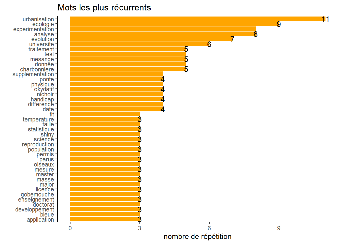
If you look carefully at the code you will see that I have made lemmatisation, that is, I have sought to exploit the meaning of the words and not the word as such.
For example, analyst, analyze or analysis have the same meaning for me of analysis so I have grouped them under the same word.
There may be an official list for lemmatisation, but I don’t know it, sorry!
Bigram measurement
A single word does not always mean something, hence the need to use n-grammms as well (here I would stop at the bigram, but it is of course possible to search for the number of words you want!).
# Creation of the bigram file for expressions
bigram <- curriculum %>%
  mutate(texte = texte %>%
           str_remove_all("\\d") %>%
           str_replace_all("[:punct:]", " ") %>%
           chartr(old = "àâäçéèêëîïôöùûüÿ",
                  new = "aaaceeeeiioouuuy")
         ) %>%
  unnest_tokens(bigramme, texte, token = "ngrams", n = 2) %>%
  separate(bigramme, c("mot1", "mot2"), sep = " ") %>%
  filter(!mot1 %in% (stop_words_fr$mot %>% chartr(old = "àâäçéèêëîïôöùûüÿ", new = "aaaceeeeiioouuuy"))) %>%
  filter(!mot2 %in% (stop_words_fr$mot %>% chartr(old = "àâäçéèêëîïôöùûüÿ", new = "aaaceeeeiioouuuy"))) %>%
  filter(!mot1 %in% (stop_words$word %>% chartr(old = "àâäçéèêëîïôöùûüÿ", new = "aaaceeeeiioouuuy"))) %>%
  filter(!mot2 %in% (stop_words$word %>% chartr(old = "àâäçéèêëîïôöùûüÿ", new = "aaaceeeeiioouuuy"))) %>%
  select(- page) %>%
  mutate_all(
    ~ str_remove_all(., "s$") %>%
      str_replace_all(
        c(
          "analys\\w+" = "analyse",
          "biostatistique" = "statistiques",
          "automatiser" = "automatisation",
          "experi\\w+" = "experimentation",
          "evolutive" = "evolution",
          "urba\\w+" = "urbanisation",
          "universit\\w+" = "universite",
          "permi" = "permis",
          "paru" = "parus",
          "ox[iy]d\\w+" = "oxydatif"))
    ) %>%
  unite(bigramme, mot1, mot2, sep = " ") %>%
  count(bigramme, sort = TRUE)

#  and graphic representation
bigram %>%
  filter(n > 1) %>%
  ggplot() +
  aes(reorder(bigramme, n), n) +
  geom_bar(stat = "identity", fill = "cyan") +
  geom_text(
    aes(label= as.character(n)),
    check_overlap = TRUE,
    size = 4) +
  coord_flip() +
  xlab(" ") +
  ylab("nombre de répétition") +
  labs(title = "Expressions les plus utilisées") +
  theme_classic()
Creation of the word cloud
I chose to remove some of the bigrams because they don’t mean anything.
# Creation of the list of words/expression to represent

liste_nuage_de_mots <- tibble(
  mot_expression = (bigram %>% filter(n >1))$bigramme,
  frequence = (bigram %>% filter(n >1))$n) %>%
  add_row(
    mot_expression = "test post hoc",
    frequence = 2) %>%
  filter(
    ! mot_expression %in% c(
      "traitement froid",
      "tit parus",
      "post hoc",
      "test post",
      "mieux comprendre",
      "major journal",
      "intensite locale",
      "evolution universite"
    )
  )

# Be careful, you must remove from single words the words already present in the bigram

liste_nuage_de_mots %<>%
  bind_rows(
    texte %>%
      filter(n > 2) %>%
      anti_join(
        liste_nuage_de_mots %>%
          separate(
            mot_expression,
            c("mot1", "mot2"),
            sep = " ") %>%
          select(- frequence) %>%
          gather("position", "mot") %>%
          select(mot)
      ) %>%
      rename("mot_expression" = "mot",
             "frequence" = "n")
  )

set.seed(1111)
wordcloud::wordcloud(words = liste_nuage_de_mots$mot_expression,
          freq = liste_nuage_de_mots$frequence,
          min.freq = 1,
          random.order = FALSE,
          colors = c( "#FF7F24", "#00F5FF", "#9400D3", "#FFD700", "#00CD00"))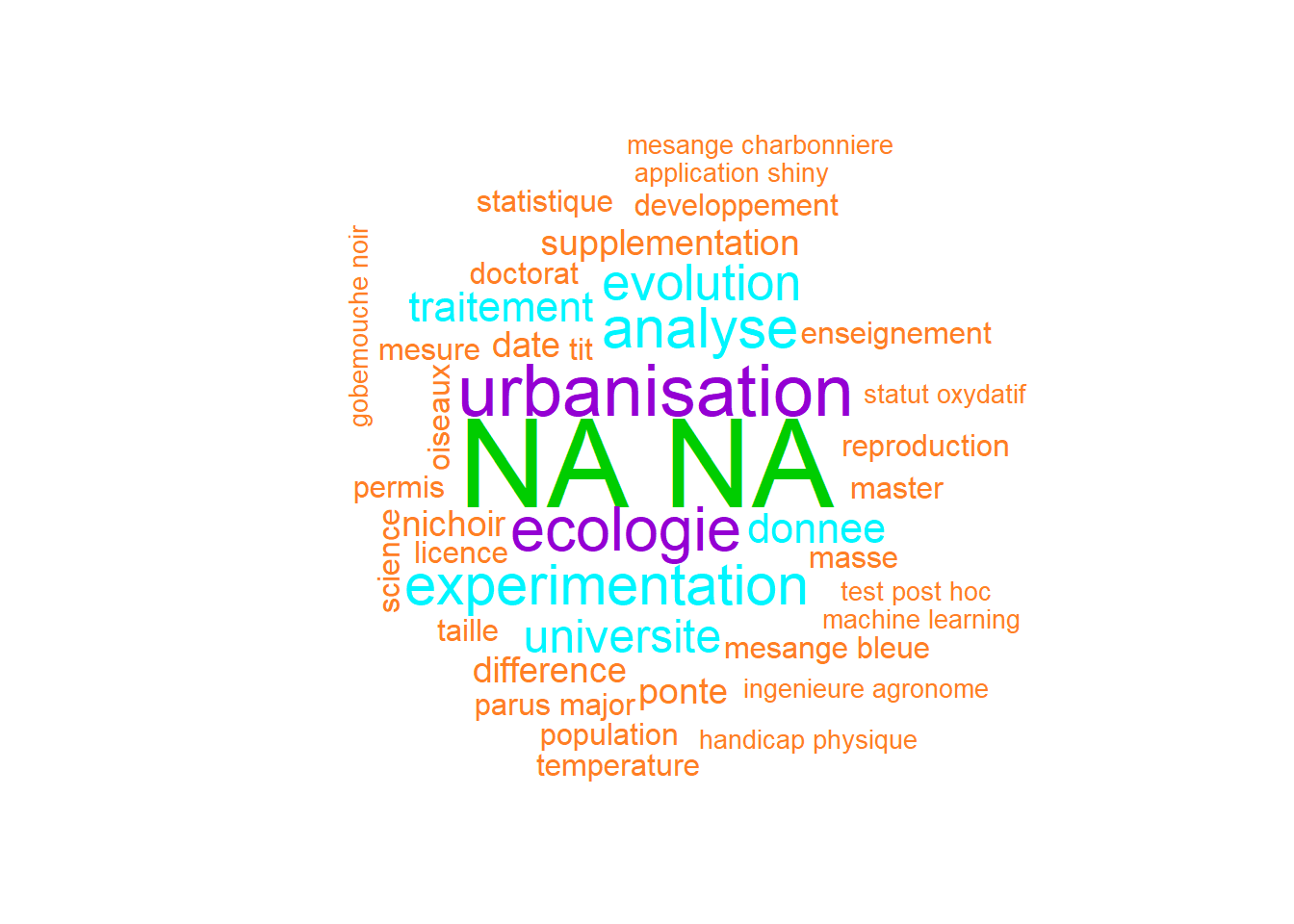
wordcloud2::wordcloud2(
  liste_nuage_de_mots,
  fontWeight = 'normal',
  color = 'random-light')
Conclusion
There you go!
So what do you think about it?
I’m quite happy to see the result. ^ ^
Share this post
Twitter
Google+
Facebook
Reddit
LinkedIn
StumbleUpon
Pinterest
Email