Automatic generation and dispatch of media to customers, blocking points and forwarding solutions
Article from the presentation that should have been made for the International Women's Day in Nantes on March 19 and which was cancelled due to the COVID-19 outbreak
Aim
The aim is to create a communication support for clients to see the evolution of their results compared to the data of other clients in the same category (Benchmark).
This support had to be generated and sent automatically to the customers.
So that people who wish to reuse these lines of code, the template used is here, the data are those of the Penguins of the package FlexParamCurve by Stephen OSWALD and LifeCycleSavings of the package datasets. Examples of the published media at the end of the article are available here and here.
Work sequence:
_ Creation of a template under Power Point
_ Creation of the graphics to be inserted
_ Creation Power Point support using the officer package from David Gohel
_ Sending support with sendmailR from Olaf Mersmann
Creating graphs on the data
When I carried out this work it was on customer data and therefore confidential. For this blog post I’m going to use the mass data of penguins according to their ages and compare it to the average data of other penguins born in the same order and the same year to show how to make a graph with a benchmark. I’m also going to do another graph on the international data of real disposable income per capita.
Comparison of one penguin to another
Comparing a penguin to others of the same year and birth order is easy with ggplot.
library(tidyverse)
library(FlexParamCurve) # to get the data on the penguins

creation_of_the_graph_for_comparing_a_penguin_to_others <- function(num_penguin){

  benchmarck <- penguin.data %>%
    filter(
      bandid != num_penguin,
      year == (penguin.data %>% filter(bandid == num_penguin) %>% slice(1))$year,
      ck == (penguin.data %>% filter(bandid == num_penguin) %>% slice(1))$ck
    ) # Benchmarking is done with data from other penguins born in the same year and in the same hatching order

  penguin.data %>%
    filter(
      bandid == num_penguin
    ) %>%
    ggplot() +
    aes(
      x = ckage,
      y = weight
    ) +
    geom_smooth(data = benchmarck, color = "red", fill = "orange", alpha = 0.4, formula = y ~ x^2) +
    geom_point(color = "black") +
    geom_smooth(se = FALSE, formula = y ~ x^2, color = "black") +
    theme_classic() +
    ggtitle(glue::glue("Penguin '{num_penguin}' compare to his peers (in red)"))

 }

"-0.993421052631561 422" %>%
  creation_of_the_graph_for_comparing_a_penguin_to_others()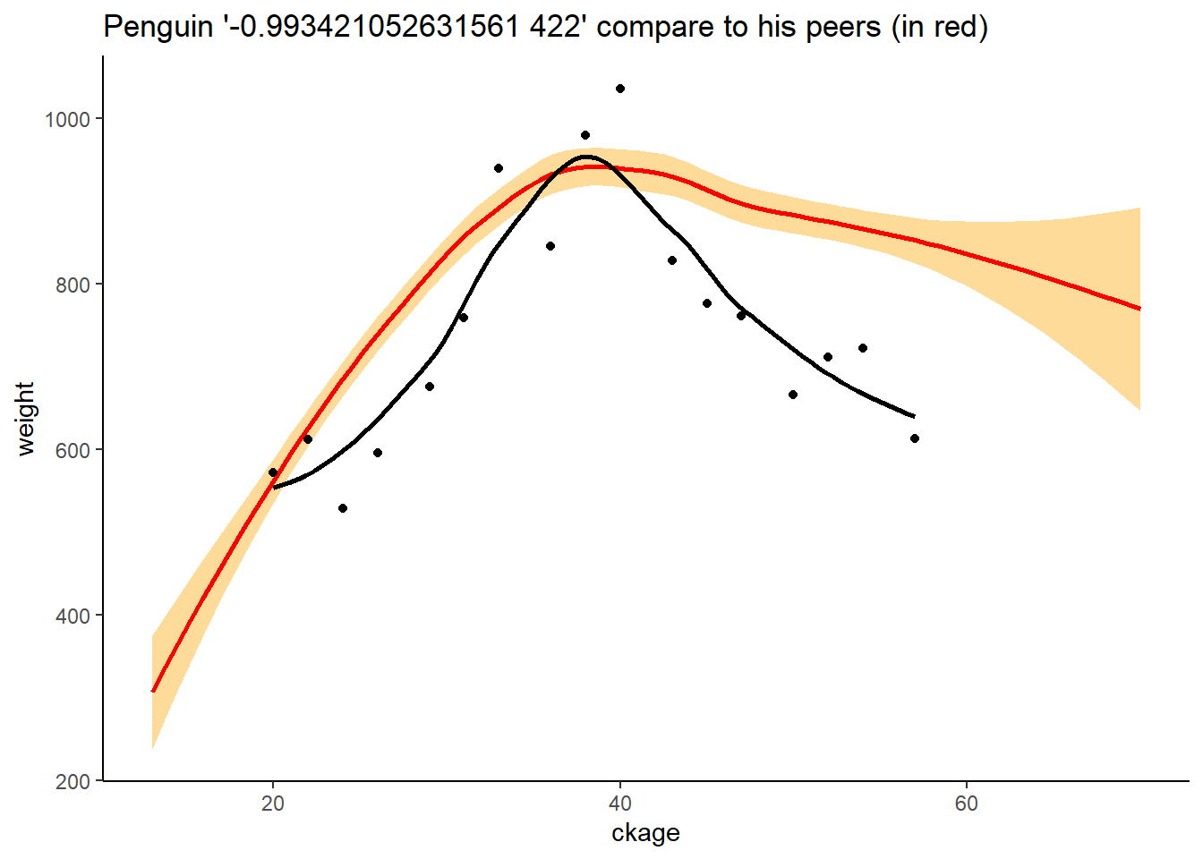
"-0.993421052631561 308" %>%
  creation_of_the_graph_for_comparing_a_penguin_to_others()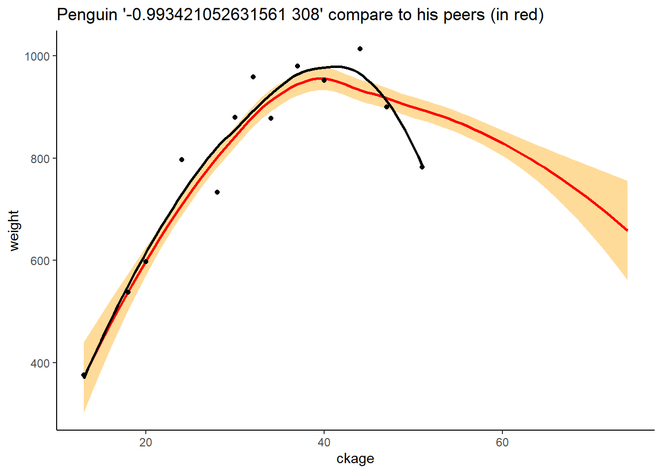
Creating a function to view data in “French” format
Basically, R presents numerical data without spaces or rounding but from time to time in graphs, it may be interesting to be able to display the figures in “French” format i.e. 123 456 789 as Excel can do natively.
For this example, I will use the data from LifeCycleSavings.
# library(tidyverse) # not useful if already called previously
library(scales) # to use the label_number function for number formatting
library(ggrepel) # to add non-overlapping values to the chart

fr_formatting <- label_number(accurancy = 1)
# I ask that there be no decimal point

# it works
1332859475.645878 %>% fr_formatting()
## [1] "1 332 859 476"LifeCycleSavings %>%
rownames_to_column("country") %>%
mutate(label = dpi %>% fr_formatting()) %>%
ggplot() +
aes(x = country, y = dpi) +
geom_segment(aes(xend = country, y = 0, yend = dpi), size = 6) +
geom_label_repel(aes(label = label), segment.color = NA, direction="y", size = 3) +
theme_classic() +
theme(
axis.text.x = element_text(angle = 90)
)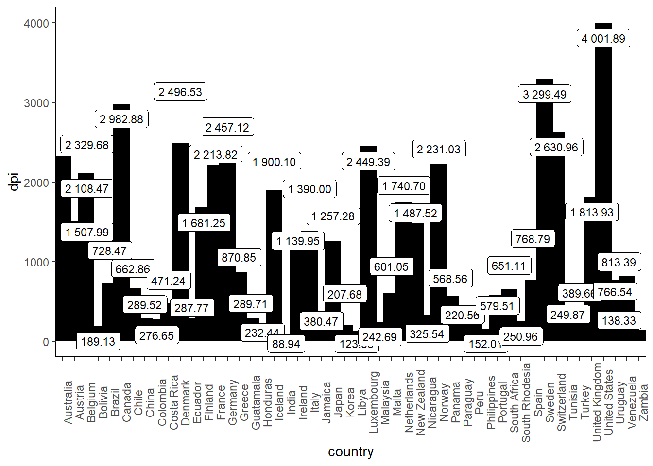
# ouch the rounding is not doneYou can see that despite my preliminary test, it doesn’t work well…
Indeed, if the global formatting is good, the rounding is not done… But why????
I was stuck for a while wondering what was wrong and why and ended up asking for help on the French slack of R users, GRRR.
Little info point: Whatever media you want to ask for help on, think about making a repex, a reproducible example!
Yes, people on the forums or slacks are your friends and yes, the R sphere is benevolent but don’t forget that nobody is in your head (except you, at least normally), so the first step towards solving a problem is to take it out of context so that you can explain it to everyone using accessible data!
This has already happened to me more than once that when I did my repex to ask for help I saw where the problem was.
Here are the lines of code I shared on the slack.
# library(scales)
# library(tidyverse)

fr_formatting <- label_number(accurancy = 1)

c(13556.4646, 546946.65465) %>% map(fr_formatting)
## [[1]]
## [1] "13 556"
##
## [[2]]
## [1] "546 947"tibble(
valeur =
runif(n = 50, min = 100, max = 6000)
) %>%
mutate(mise_en_forme = valeur %>% fr_formatting)## # A tibble: 50 x 2
## valeur mise_en_forme
## <dbl> <chr>
## 1 3172. 3 171.79
## 2 5331. 5 331.45
## 3 4319. 4 319.15
## 4 1053. 1 053.26
## 5 2587. 2 587.38
## 6 4182. 4 182.38
## 7 4941. 4 941.50
## 8 3855. 3 854.62
## 9 2109. 2 109.46
## 10 2764. 2 764.42
## # ... with 40 more rowsThis time it was Julien Barnier who helped me out by pointing out that I had made a mistake at accuracy, there is no ‘n’….
Strangely enough, it worked better right away.
fr_formatting <- label_number(accuracy = 1)
tibble(
  valeur =
    runif(n = 50, min = 100, max = 6000)
  ) %>%
  mutate(mise_en_forme = valeur %>% fr_formatting)
## # A tibble: 50 x 2
## valeur mise_en_forme
## <dbl> <chr>
## 1 4190. 4 190
## 2 5807. 5 807
## 3 848. 848
## 4 4264. 4 264
## 5 4575. 4 575
## 6 4906. 4 906
## 7 3087. 3 087
## 8 3035. 3 035
## 9 4490. 4 490
## 10 1576. 1 576
## # ... with 40 more rowsgraphique_LCS <- LifeCycleSavings %>%
rownames_to_column("country") %>%
mutate(label = dpi %>% fr_formatting()) %>%
ggplot() +
aes(x = country, y = dpi) +
geom_segment(aes(xend = country, y = 0, yend = dpi), size = 6) +
geom_label_repel(aes(label = label), segment.color = NA, direction="y", size = 3) +
theme_classic() +
theme(
axis.text.x = element_text(angle = 90)
)
graphique_LCS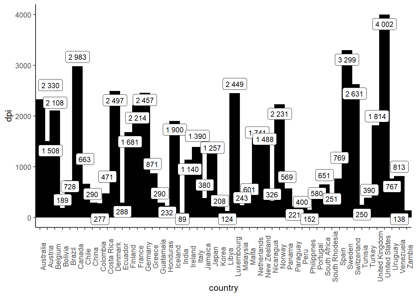
Creating PowerPoint support with officer
Basically I’m not too much for creating pptx support with R, I prefer html reports but it is still a much awaited support for communication to customers.
With the officer package, I will create simple but dynamic support with links between slides.
library(officer)
library(glue)

location_of_support <- "template_rstudio_article_off_eng.pptx"

# pour voir les types de diapos qui existent et les éléments qui les constituent
read_pptx(location_of_support) %>%
  layout_properties() %>%
  select(master_name, name, type, id, ph_label)
## master_name name type id ph_label
## 1 Intégral Diapositive de titre body 10 Rectangle 9
## 2 Intégral Diapositive de titre body 8 Straight Connector 7
## 3 Intégral Diapositive de titre body 12 ZoneTexte 11
## 4 Intégral Diapositive de titre body 11 Oval 5
## 5 Intégral Contenu avec légende body 3 Content Placeholder 2
## 6 Intégral Contenu avec légende body 4 Text Placeholder 3
## 7 Intégral Contact body 26 ZoneTexte 25
## 8 Intégral Contact body 22 Image 21
## 9 Intégral Image avec légende body 4 Text Placeholder 3
## 10 Intégral Image avec légende body 8 Straight Connector 7
## 11 Intégral Resume body 10 Espace réservé du texte 9
## 12 Intégral Titre et texte vertical body 3 Vertical Text Placeholder 2
## 13 Intégral Resume body 14 Espace réservé du texte 13
## 14 Intégral Titre vertical et texte body 3 Vertical Text Placeholder 2
## 15 Intégral Titre vertical et texte body 7 Straight Connector 6
## 16 Intégral Contact body 14 ZoneTexte 13
## 17 Intégral Resume body 22 Espace réservé du texte 21
## 18 Intégral Contact body 23 Rectangle 22
## 19 Intégral Contact body 24 Rectangle 23
## 20 Intégral Resume body 6 Espace réservé du texte 5
## 21 Intégral Contact body 3 ZoneTexte 2
## 22 Intégral Contact body 8 Graphique 7
## 23 Intégral Contact body 12 Espace réservé du contenu 5
## 24 Intégral Titre, Contenu et Image body 6 Espace réservé du contenu 5
## 25 Intégral Resume body 12 Espace réservé du texte 11
## 26 Intégral Titre, Contenu et Image body 9 Espace réservé du contenu 8
## 27 Intégral Resume body 16 Espace réservé du texte 15
## 28 Intégral Resume body 18 Espace réservé du texte 17
## 29 Intégral Resume body 20 Espace réservé du texte 19
## 30 Intégral Titre et contenu body 6 Espace réservé du contenu 5
## 31 Intégral Resume body 24 Espace réservé du texte 23
## 32 Intégral Resume body 4 Rectangle 3
## 33 Intégral Comparaison body 5 Text Placeholder 4
## 34 Intégral Titre, Contenu et Image body 5 Graphique 4
## 35 Intégral Titre de section body 8 Straight Connector 7
## 36 Intégral Titre, Contenu et Image body 7 Espace réservé du contenu 6
## 37 Intégral PrésentationMarie body 7 ZoneTexte 6
## 38 Intégral Titre, Contenu et Image body 4 Espace réservé du contenu 3
## 39 Intégral PrésentationMarie body 8 Espace réservé du contenu 5
## 40 Intégral Titre de section body 9 Rectangle 8
## 41 Intégral Titre et contenu body 3 Content Placeholder 2
## 42 Intégral Titre et contenu body 4 Graphique 3
## 43 Intégral Titre de section body 3 Text Placeholder 2
## 44 Intégral Comparaison body 6 Content Placeholder 5
## 45 Intégral Titre de section body 11 Oval 5
## 46 Intégral Deux contenus body 3 Content Placeholder 2
## 47 Intégral PrésentationMarie body 4 Graphique 3
## 48 Intégral PrésentationMarie body 3 ZoneTexte 2
## 49 Intégral Comparaison body 4 Content Placeholder 3
## 50 Intégral Deux contenus body 4 Content Placeholder 3
## 51 Intégral Comparaison body 3 Text Placeholder 2
## 52 Intégral Titre et contenu title 2 Title 1
## 53 Intégral Titre, Contenu et Image title 2 Title 1
## 54 Intégral Image avec légende title 2 Title 1
## 55 Intégral Contenu avec légende title 8 Title 7
## 56 Intégral Titre vertical et texte title 2 Vertical Title 1
## 57 Intégral Deux contenus title 2 Title 1
## 58 Intégral Titre et texte vertical title 2 Title 1
## 59 Intégral Titre de section title 2 Title 1
## 60 Intégral Comparaison title 10 Title 9
## 61 Intégral Titre seul title 2 Title 1
## 62 Intégral Diapositive de titre ctrTitle 2 Title 1
## 63 Intégral Diapositive de titre tbl 5 Espace réservé du tableau 4
## 64 Intégral Image avec légende pic 3 Picture Placeholder 2creating_support <- function(num_penguin){
read_pptx(location_of_support) %>%
# 1. Creating the title slide
add_slide(
layout = "Diapositive de titre",
master = "Intégral"
) %>%
ph_with(
value = num_penguin,
location = ph_location_label("Title 1")
) %>%
ph_with(
value = penguin.data %>% filter(bandid == num_penguin) %>% slice(1) %>% as_tibble() %>% select(year, ck),
location = ph_location_label("Espace réservé du tableau 4")
) %>%
# 2. Adding clickable summary
add_slide(
layout = "Resume",
master = "Intégral"
) %>%
ph_with(
value = glue("Penguin identification number : {num_penguin}"),
location = ph_location_label("Espace réservé du texte 5")
) %>%
ph_with(
value = "Information about Marie Vaugoyeau",
location = ph_location_label("Espace réservé du texte 9")
) %>%
ph_with(
value = "Graphique Life Cycle Saving",
location = ph_location_label("Espace réservé du texte 11")
) %>%
ph_with(
value = glue("Graph associated with the penguin {num_penguin}"),
location = ph_location_label("Espace réservé du texte 13")
) %>%
ph_with(
value = "Contact information",
location = ph_location_label("Espace réservé du texte 15")
) %>%
# 3. Addition of the information slide about me (small ad page)
add_slide(
layout = "PrésentationMarie",
master = "Intégral"
) %>%
ph_with(
value = "Click back to the menu",
location = ph_location_label("Espace réservé du contenu 5")
) %>%
ph_slidelink(
ph_label = "Espace réservé du contenu 5",
slide_index = 2
) %>%
# 4. Adding LCS graph
add_slide(
layout = "Titre et contenu",
master = "Intégral"
) %>%
ph_with(
value = "Graph LCS",
ph_location_label("Title 1")
) %>%
ph_with(
value = graphique_LCS,
ph_location_label("Content Placeholder 2")
) %>%
ph_with(
value = "Click back to the menu",
location = ph_location_label("Espace réservé du contenu 5")
) %>%
ph_slidelink(
ph_label = "Espace réservé du contenu 5",
slide_index = 2
) %>%
# 5. Adding custom penguin graphic
add_slide(
layout = "Titre, Contenu et Image",
master = "Intégral"
) %>%
ph_with(
value = "Penguin graph",
ph_location_label("Title 1")
) %>%
ph_with(
value = external_img("pingouin.png"), # image extraite de l'article à l'origine des données
location = ph_location_label("Espace réservé du contenu 3")
) %>%
ph_with(
value = glue("{(penguin.data %>% filter(bandid == num_penguin) %>% slice(1))$year} {(penguin.data %>% filter(bandid == num_penguin) %>% slice(1))$ck}"),
ph_location_label("Espace réservé du contenu 8")
) %>%
ph_with(
value = creation_of_the_graph_for_comparing_a_penguin_to_others(num_penguin),
ph_location_label("Espace réservé du contenu 6")
) %>%
ph_with(
value = "Click back to the menu",
location = ph_location_label(ph_label = "Espace réservé du contenu 5")
) %>%
ph_slidelink(
ph_label = "Espace réservé du contenu 5",
slide_index = 2
) %>%
# 6. Adding the contact slide
add_slide(
layout = "Contact",
master = "Intégral"
) %>%
ph_with(
value = "Click back to the menu",
location = ph_location_label(ph_label = "Espace réservé du contenu 5")
) %>%
ph_slidelink(
ph_label = "Espace réservé du contenu 5",
slide_index = 2
) %>%
# Creating links on the contents page
on_slide(index = 2) %>%
ph_slidelink(
ph_label = "Espace réservé du texte 9",
slide_index = 3
) %>%
ph_slidelink(
ph_label = "Espace réservé du texte 11",
slide_index = 4
) %>%
ph_slidelink(
ph_label = "Espace réservé du texte 13",
slide_index = 5
) %>%
ph_slidelink(
ph_label = "Espace réservé du texte 15",
slide_index = 6
)
}Sending the support with the package sendmailR
Once the skeleton of the support is ready, all that’s left to do is to send each penguin (or each client) his personalized support.
library(sendmailR)

num_penguin <- c("-0.993421052631561 422", "-0.993421052631561 308")

message_support <- map(
  .x = num_penguin,
  .f = ~ mime_part(
    creating_support(.x),
    "support.pptx"
  )
)

message_support[[1]]$`Content-Type` <- "application/vnd.openxmlformats-officedocument.presentationml.presentation"

message_support[[2]]$`Content-Type` <- "application/vnd.openxmlformats-officedocument.presentationml.presentation"

shipping_address <- c("experimentatateur1@truc.com", "experimentateur2@truc.com") # address of the person who followed the penguin/customer

penguin_address <- c("pingouin1@pole_nord.fr", "pingouin2@pole_nord.fr") # email address of the penguin/customer

# Sending emails
map2(
  .x = shipping_address,
  .y = penguin_address,
  .f = ~ sendmail(
    from = glue("<{.x}>"),
    to = glue("<{.y}>"),
    subject = glue("Synthesis of penguin weight gain {num_penguin}"),
    msg = list(
      glue("Hello,\nPlease find attached the synthesis for the penguin {num_penguin}.\nHave a nice day, \nMarie Vaugoyeau"),
      message_support
    ),
    control = list(smtpServer = "ASPMX.L.GOOGLE.COM")
  )
)
Oops, it doesn’t work…
But why??
In fact, a quick phone call to David Gohel, 1 minute of conversation and hop the solution is obvious, what I treat as a pptx is in fact an rpptx….
So you have to edit the pptx support before sending it and then it’s ok !
Two solutions, either we save all the pptx supports we send for archive (solution taken here and here), or we create a temporary support which will be overwritten.
pptx_support_recording <- function(num_penguin){
  num_penguin %>%
    creating_support() %>%
    print(glue('presentation_{num_penguin %>% str_remove_all("[:punct:]")}_eng.pptx'))
}

num_penguin <- c("-0.993421052631561 422", "-0.993421052631561 308")

num_penguin %>%
  map(pptx_support_recording)
There you go!
I hope that this article will help you better seek help and make your work with R easier.
Twitter
Google+
Facebook
Reddit
LinkedIn
StumbleUpon
Pinterest
Email