First step: Outliers and Boxplot

Before to start anything, I test the data to find outliers (observation that has a relatively large or small value compared to the majority of observations Zuur et al. (2010)).

I start by draw boxplots by month (one by characteristic).

library(ggplot2)
for (i in 3:6)
{
bp<-ggplot(X) + geom_boxplot(aes(x = as.factor(Date), y = X[,i])) + geom_jitter(aes(x = as.factor(Date), y = X[,i]), col = X$Site, alpha = 0.2) + theme_minimal() + xlab("Date") + ylab(variable.names(X)[i])
print(bp)
}

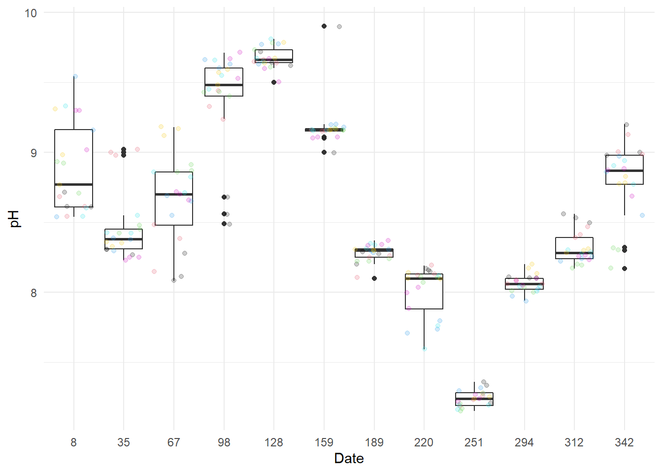
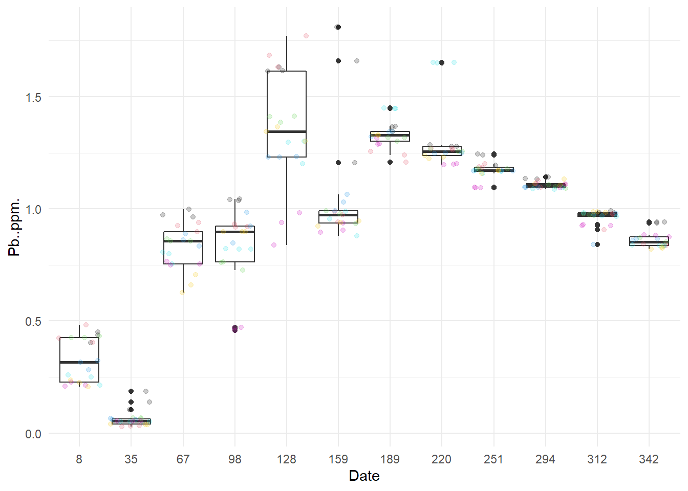
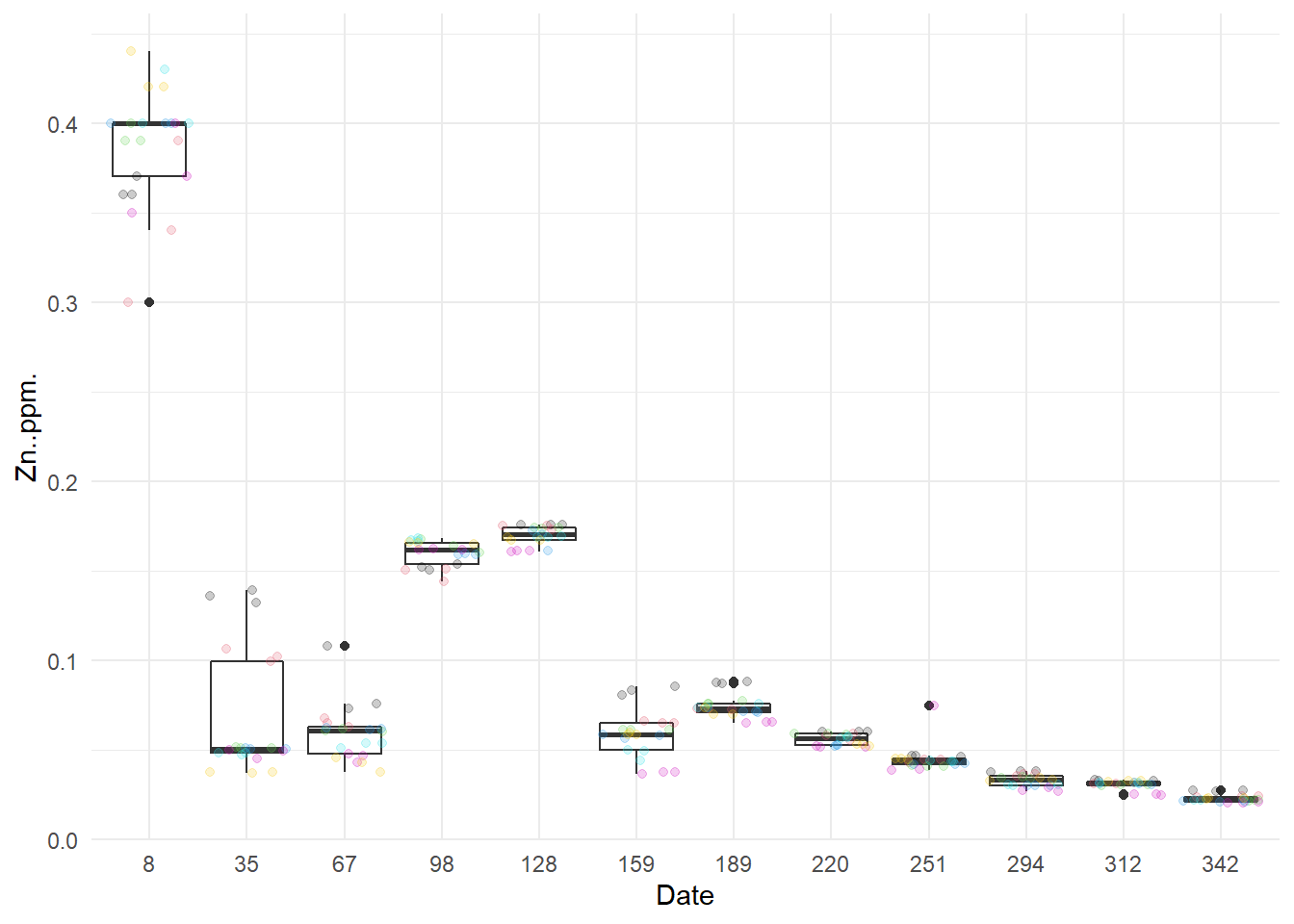
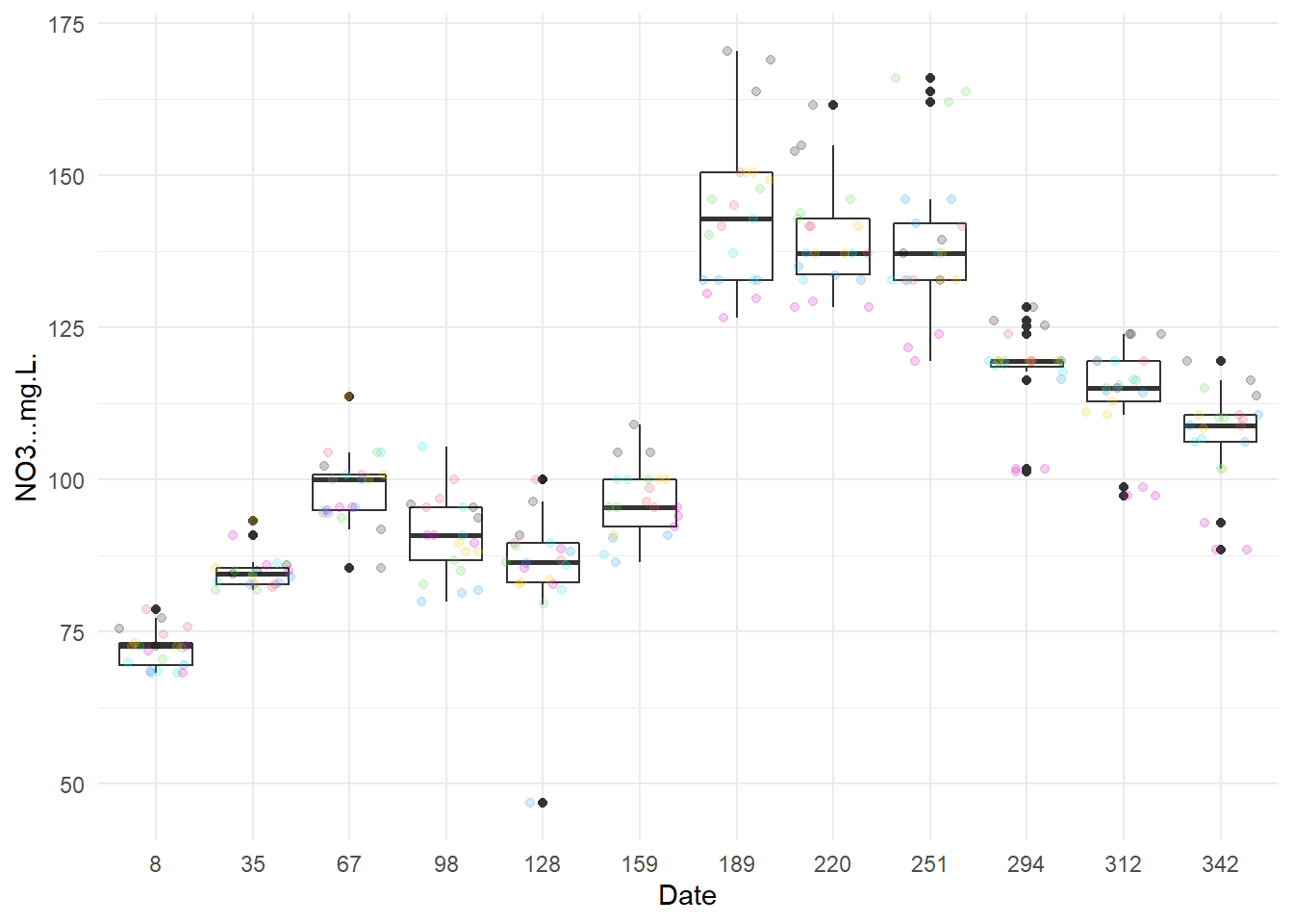Except for NO₃^- at 128 days after the start of the year, there does not seem to have any outlier.

Second step: Outliers, means and standard error

In the data used, measurements were did three times each, so I calculated means and standard error with plotrix library.

library(plotrix)

X$rep<-paste(as.factor(X$Site), as.factor(X$Date))
# I create a variable to work on the repetition of measurements

# I create also the new database Z to have means and standard error according to spot and date
Site<-rep(1:7, each = 12)
Date<-rep(c(128,159,189,220,251,294,312,342,35,67,8,98), 7)
Z<-cbind(Site,Date)
CN<-colnames(Z)

for (i in 3:6)
{
M<-tapply(X[,i], X$rep, mean, na.rm=TRUE)
S<-tapply(X[,i], X$rep, std.error, na.rm=TRUE)
Z<-cbind(Z, M, S)
CN<-c(CN, paste(variable.names(X)[i],"Mean"),paste(variable.names(X)[i],"Se"))
}

colnames(Z)<-CN

write.table(Z, row.names=FALSE, "Physicochimical.txt", sep=";")
# Exporte table to work on it later

Then I analyse standard error by drawing.

Z<-read.table("Physicochimical.txt", header = TRUE, sep = ";")
o <- order(Z$Date)
Z<-Z[o,]
Z$Site<-as.factor(Z$Site)

for (i in c(4,6,8,10))
{
  se<-ggplot(Z) + geom_point(aes(x = Date, y = Z[,i], color = Site)) + theme_minimal() + xlab("Date") + ylab(variable.names(Z)[i])
  print(se)
}

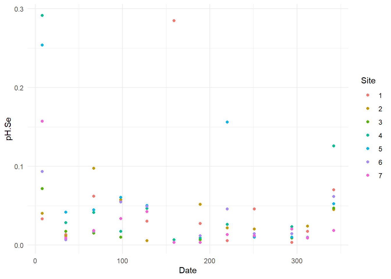
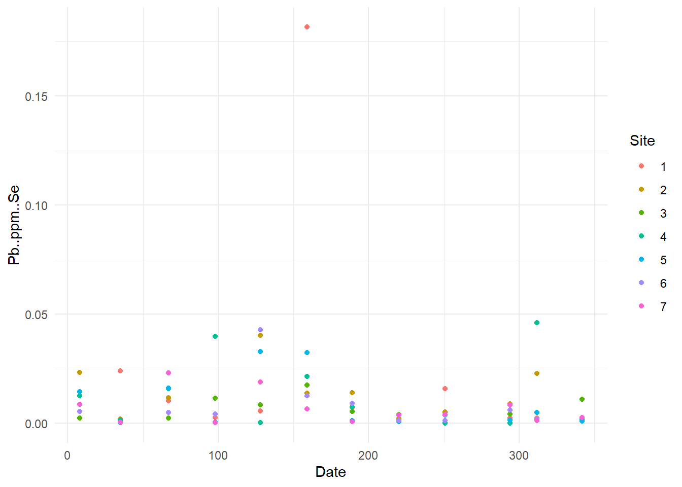
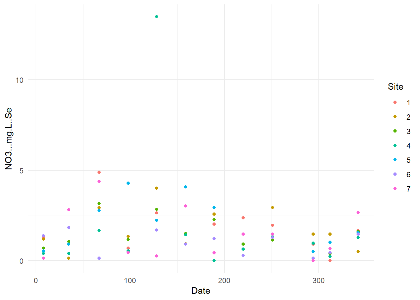Now, we can see some standard error were higher than other (example for Pb one point has error higher than 0.1), so I will verify these specific data.
This method allows me to found and correct five misprint in the data. I will take in mind other outlier to check their influences on the futur analyses.