My first article: A not fully crossed design
Statistical analyses for my first article published

In 2015, I published the article: Is oxidative status influenced by dietary carotenoid and physical activity after moult in the great tit (Parus major)? about my first experimentation. In the aim to investigate on the relationship between dietary carotenoids, physical activity and oxidative status, I captured great tits and kept them in aviaries.
Initially, a cross design: with/without dietary carotenoids and with/without plucking primary feathers (to increase physical activity or not), was planned. Due to weather conditions, number of caught birds was to low to do it, so only three treatments were done.
| Dietary carotenoids in water | Natural water | |
|---|---|---|
| Physical activity increased | 7F 7M | 7F 7M |
| Normal physical activity | 7F 7M | 7F 7M |
With F = females and M = males
Unfortunately, I caught only 42 adults (1 was dead before the beginning of the experiment).
| Dietary carotenoids in water | Natural water | |
|---|---|---|
| Physical activity increased | 6F 8M | 5F 8M |
| Normal physical activity | 7F 7M |
Here I detail the statistical analyses that I did it.
First Step: Check the repeatability of the data
For some characteristics (counts heterophiles on lymphocytes, feathers colour…), I did two, three or four measurements. To measure repeatability, I used a linear model which give me F-statistic with freedom degree and p-value.
mod<-lm(Area~Identity, data=X)
anova(mod)
## Analysis of Variance Table
##
## Response: Area
## Df Sum Sq Mean Sq F value Pr(>F)
## Identity 1 11.558 11.5584 10.346 0.001655 **
## Residuals 124 138.528 1.1172
## ---
## Signif. codes: 0 '***' 0.001 '**' 0.01 '*' 0.05 '.' 0.1 ' ' 1In this article, I also calculated manually intraclass correlation coefficient according Lessells and Boag’s method 1987: r = (MSA - MSw)/(MSA + MSW(n-1)).
Once repeatability was checked, I calculated and used only means.
Second step: Linear mixed models with backward elimination
In order to test the effects of physical activity and dietary carotenoid availability on the antioxidant system (total antioxidant capacity, ROM concentration, total carotenoids, vitamin A and vitamin E), on the stress response (blood sedimentation and H/Ly ratio) and on plumage colour (lutein absorbance, carotenoid chroma and UV brightness), all models included as fixed effects tarsus length and body mass, and three-way interactions among carotenoid supplementation or physical handicap with sex and time of experiment (start or end of the experiment).
Linear mixed model
For each variable, I write a mixed model like that:
library(nlme)
m1<-lme(Oxy ~ Tarsus+Mass+Exp*Sex*Carot+Exp*Sex*Plucking, random=list(Aviary=~1, Identity=~1), method="ML", data = Y, na.action=na.exclude)
To consider biological variance, aviaries and individual identity were included as random factors.
Distribution of model residuals
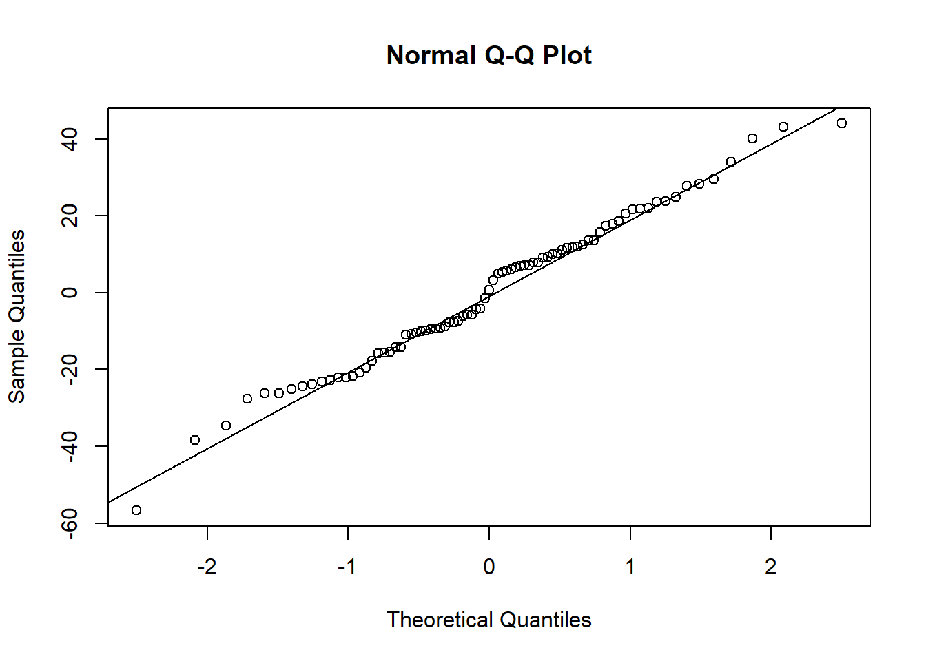
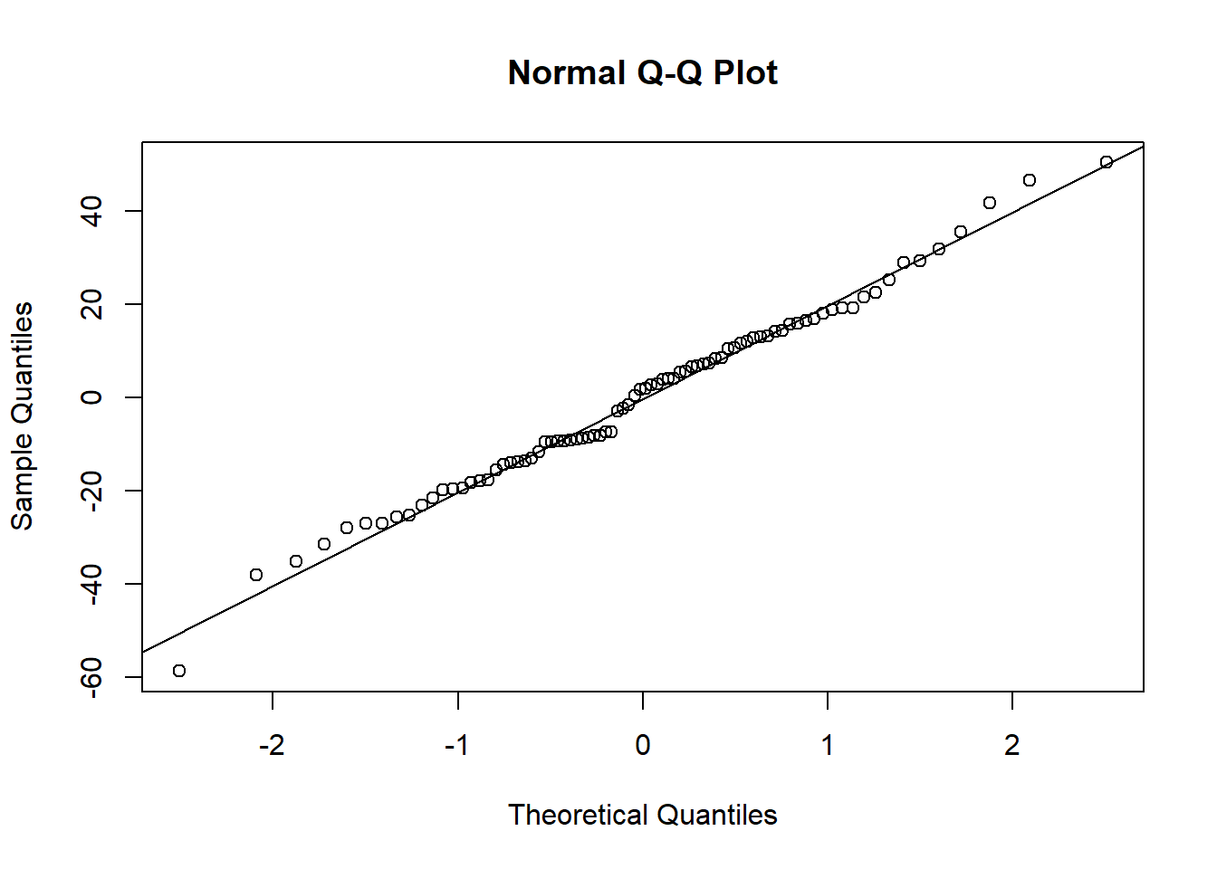
To validate a posteriori the used of linear model, I tested residuals distribution with Shapiro test and Q-Q plot.
shapiro.test(residuals(m1))##
## Shapiro-Wilk normality test
##
## data: residuals(m1)
## W = 0.98678, p-value = 0.5759qqnorm(residuals(m1));qqline(residuals(m1)) If residuals did not follow normal distribution, variable was log-transformed.
Model selection with backward elimination
About first model, I created a new one by removing one fixed factor. Then, I used Akaike’s Information Criterion to select the best predictive model between both.
anova(m1)## numDF denDF F-value p-value
## (Intercept) 1 33 3894.578 <.0001
## Tarsus 1 25 9.314 0.0053
## Mass 1 33 0.414 0.5243
## Exp 1 33 37.679 <.0001
## Sex 1 25 5.208 0.0313
## Carot 1 9 0.519 0.4897
## Plucking 1 9 1.001 0.3432
## Exp:Sex 1 33 0.888 0.3529
## Exp:Carot 1 33 2.560 0.1191
## Sex:Carot 1 25 0.017 0.8986
## Exp:Plucking 1 33 1.918 0.1753
## Sex:Plucking 1 25 2.002 0.1694
## Exp:Sex:Carot 1 33 0.113 0.7391
## Exp:Sex:Plucking 1 33 0.782 0.3831summary(m1)## Linear mixed-effects model fit by maximum likelihood
## Data: Y
## AIC BIC logLik
## 772.4558 813.1614 -369.2279
##
## Random effects:
## Formula: ~1 | Aviary
## (Intercept)
## StdDev: 7.01982
##
## Formula: ~1 | Identity %in% Aviary
## (Intercept) Residual
## StdDev: 7.071078 21.21047
##
## Fixed effects: Oxy ~ Tarsus + Mass + Exp * Sex * Carot + Exp * Sex * Plucking
## Value Std.Error DF t-value p-value
## (Intercept) 289.61059 143.81205 33 2.013813 0.0522
## Tarsus -3.63000 6.48630 25 -0.559640 0.5807
## Mass -0.09082 4.43841 33 -0.020462 0.9838
## ExpStart 44.13499 13.03342 33 3.386293 0.0018
## SexM -14.94850 15.46285 25 -0.966736 0.3429
## CarotYes -1.46163 16.34930 9 -0.089400 0.9307
## PluckingYes 23.53261 15.67578 9 1.501208 0.1675
## ExpStart:SexM 5.54477 18.34549 33 0.302241 0.7644
## ExpStart:CarotYes -11.31881 19.99812 33 -0.565994 0.5752
## SexM:CarotYes 10.80621 20.00440 25 0.540192 0.5938
## ExpStart:PluckingYes -5.26320 19.44272 33 -0.270703 0.7883
## SexM:PluckingYes -9.06389 20.22299 25 -0.448197 0.6579
## ExpStart:SexM:CarotYes 4.51084 25.90055 33 0.174160 0.8628
## ExpStart:SexM:PluckingYes -23.19101 26.23251 33 -0.884056 0.3831
## Correlation:
## (Intr) Tarsus Mass ExpStr SexM CartYs PlcknY
## Tarsus -0.873
## Mass -0.247 -0.251
## ExpStart 0.031 0.073 -0.292
## SexM 0.283 -0.133 -0.381 0.497
## CarotYes 0.042 -0.144 0.205 -0.060 -0.056
## PluckingYes -0.168 0.147 -0.050 0.395 0.353 -0.558
## ExpStart:SexM -0.005 -0.056 0.182 -0.703 -0.662 0.038 -0.279
## ExpStart:CarotYes 0.013 0.013 -0.052 0.015 0.020 -0.621 0.350
## SexM:CarotYes 0.064 0.047 -0.222 0.065 0.087 -0.732 0.402
## ExpStart:PluckingYes -0.001 -0.029 0.116 -0.647 -0.303 0.366 -0.618
## SexM:PluckingYes 0.075 -0.131 0.175 -0.346 -0.656 0.417 -0.690
## ExpStart:SexM:CarotYes -0.002 -0.002 0.008 -0.002 -0.003 0.473 -0.268
## ExpStart:SexM:PluckingYes 0.001 0.036 -0.115 0.488 0.458 -0.278 0.459
## ExS:SM ExS:CY SxM:CY ExS:PY SxM:PY ES:SM:C
## Tarsus
## Mass
## ExpStart
## SexM
## CarotYes
## PluckingYes
## ExpStart:SexM
## ExpStart:CarotYes -0.009
## SexM:CarotYes -0.040 0.510
## ExpStart:PluckingYes 0.457 -0.566 -0.305
## SexM:PluckingYes 0.488 -0.278 -0.537 0.495
## ExpStart:SexM:CarotYes 0.001 -0.770 -0.649 0.433 0.339
## ExpStart:SexM:PluckingYes -0.697 0.421 0.362 -0.745 -0.672 -0.521
##
## Standardized Within-Group Residuals:
## Min Q1 Med Q3 Max
## -2.67403721 -0.67266044 0.03448938 0.58915181 2.07277186
##
## Number of Observations: 81
## Number of Groups:
## Aviary Identity %in% Aviary
## 12 41m2<-lme(Oxy ~ Tarsus+Mass+Exp*Carot+Sex*Carot+Exp*Sex*Plucking, random=list(Aviary=~1, Identity=~1), method="ML", data = Y, na.action=na.exclude)
anova(m1,m2)## Model df AIC BIC logLik Test L.Ratio p-value
## m1 1 17 772.4558 813.1614 -369.2279
## m2 2 16 770.4925 808.8036 -369.2462 1 vs 2 0.03665401 0.8482I kept the model with the smaller AIC or if difference between AIC was smaller than 2, the most parsimonious.
Final model
Final models were maximum-likelihood (REML) linear mixed models, run using the same function lme and the function Anova in the package car, with type III sum of squares.
mf<-lme(Oxy ~ Sex+Exp*Plucking, random=list(Aviary=~1, Identity=~1), method="REML", data = Y, na.action=na.exclude)
shapiro.test(residuals(mf))
##
## Shapiro-Wilk normality test
##
## data: residuals(mf)
## W = 0.99136, p-value = 0.8646qqnorm(residuals(mf));qqline(residuals(mf))
library(car)
Anova(mf, type="III")
## Analysis of Deviance Table (Type III tests)
##
## Response: Oxy
## Chisq Df Pr(>Chisq)
## (Intercept) 711.1752 1 < 2.2e-16 ***
## Sex 17.7193 1 2.560e-05 ***
## Exp 31.2056 1 2.321e-08 ***
## Plucking 5.6370 1 0.01759 *
## Exp:Plucking 4.9661 1 0.02585 *
## ---
## Signif. codes: 0 '***' 0.001 '**' 0.01 '*' 0.05 '.' 0.1 ' ' 1summary(mf)## Linear mixed-effects model fit by REML
## Data: Y
## AIC BIC logLik
## 740.8622 759.6127 -362.4311
##
## Random effects:
## Formula: ~1 | Aviary
## (Intercept)
## StdDev: 7.375749
##
## Formula: ~1 | Identity %in% Aviary
## (Intercept) Residual
## StdDev: 8.367793 22.21293
##
## Fixed effects: Oxy ~ Sex + Exp * Plucking
## Value Std.Error DF t-value p-value
## (Intercept) 211.16883 7.918474 39 26.667869 0.0000
## SexM -24.19386 5.747544 28 -4.209425 0.0002
## ExpStart 46.90000 8.395700 39 5.586193 0.0000
## PluckingYes 21.58673 9.092049 10 2.374242 0.0390
## ExpStart:PluckingYes -23.05556 10.345869 39 -2.228479 0.0317
## Correlation:
## (Intr) SexM ExpStr PlcknY
## SexM -0.363
## ExpStart -0.530 0.000
## PluckingYes -0.736 -0.054 0.462
## ExpStart:PluckingYes 0.430 0.000 -0.812 -0.569
##
## Standardized Within-Group Residuals:
## Min Q1 Med Q3 Max
## -2.64507717 -0.62459656 0.07843944 0.59250358 2.26879382
##
## Number of Observations: 82
## Number of Groups:
## Aviary Identity %in% Aviary
## 12 41Random effect
For all final model, random factors (aviaries and individual identity) were unsignificant. I tested it by the follow way:
mfR<-lme(Oxy ~ Sex+Exp*Plucking, random=list(Aviary=~1, Identity=~1), method="REML", data = Y, na.action=na.exclude)
mfNR<-gls(Oxy ~ Sex+Exp*Plucking, method="REML", data = Y, na.action=na.exclude)
anova(mfR,mfNR)
## Model df AIC BIC logLik Test L.Ratio p-value
## mfR 1 8 740.8622 759.6127 -362.4311
## mfNR 2 6 739.2564 753.3192 -363.6282 1 vs 2 2.39415 0.3021Third and last step: Analyse results
The last and a good one at that: analyse results and wrote article.
If you read until here, thank you. I remain at your disposal for questions and comments. If you want a pdf, full text is available here.


Share this post
Twitter
Google+
Facebook
Reddit
LinkedIn
StumbleUpon
Pinterest
Email